Graph all the things

analyzing all the things you forgot to wonder about

Map Projections 2: Solving Numerically

2024-02-21
interests: maps, linear algebra, machine learning

In part 1, I explained the problem of solving an optimal map projection and why we can't do it by hand. Now I'll show how I went about solving numerically and give a few teaser visualizations of the projections I designed. Results to come in the following parts!

Lore

I'm fascinated by the remote parts of the world: Baffin Island in the extreme north, Vinson Massif in the south, and the Amazon near the equator. But our map projections often make the poles look huge and shapeless while the equator is unfairly compressed.

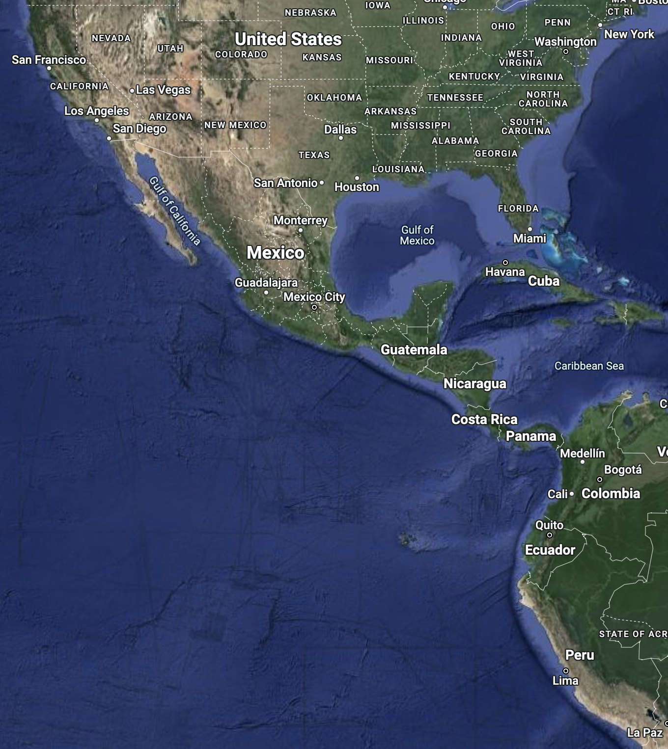
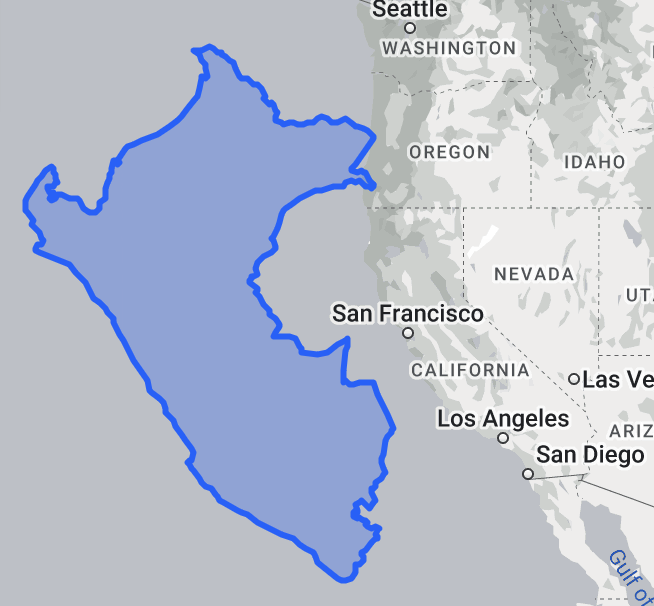
When I planned a trip to Peru several years ago, I expected it to be about the size of California. I thought I might cover the coast, Amazon, and desert in just a week and a half. But no, the Mercator projection had deceived me; Peru is 3 times as large as California. Take a look at Google's web Mercator projection (left) vs. an actual size comparison (right):

California
and Peru in the web Mercator projection

California
and Peru actual size comparison

Well, it does make sense for mapping software to use Mercator. It's computationally efficient to work with, and most importantly, it's conformal (preserves local angles everywhere). When you're giving people driving directions, it's pretty important that right angles in Alaska still look like right angles.

But my goal with designing map projections is to convey the size and shape of the planet's features as accurately as possible. That means striking a good compromise at preserving areas and angles, since doing both exactly is impossible. As non-goals: I have no interest in making lines of latitude or longitude straight, or auxiliary objectives like that.

Discretizing the globe

I made a lattice of 6,000 triangles over the globe, connecting 3,044 points. Each of these triangles has 3 angles (duh) for 18,000 angles in total. In the end, I'll sum my (weighted) local loss function evaluated at each angle.

the front of a
lattice of triangles over the globe

You can see the lattice is a bit quirky, but that helps it achieve balance:

The points are spaced so that each triangle has roughly equal area. That is, rows of points are (by default) separated by a fixed distance $dz$ in the z coordinate and a fixed angle $d\theta$ in $\theta$ .
Near the poles, I increase $d\theta$ and decrease $dz$ ; cutting the number of points per row, but increasing the number of rows. Without this, the aspect ratio of some triangles would be too long and skinny, and polar regions would lack meaningful detail.

Here's a close-up of the north pole, showing how the number of points per row cuts in half and the density of rows increases. The blue area has 50 points per row, green is a transition, and red has 25 points per row (but denser rows).

top view of
lattice of triangles over the globe

Due to topology, every map projection must have at least one interruption - one point that appears at least twice in the map. Take a look at this azimuthal projection from Wikipedia, which manages to only interrupt at the south pole:

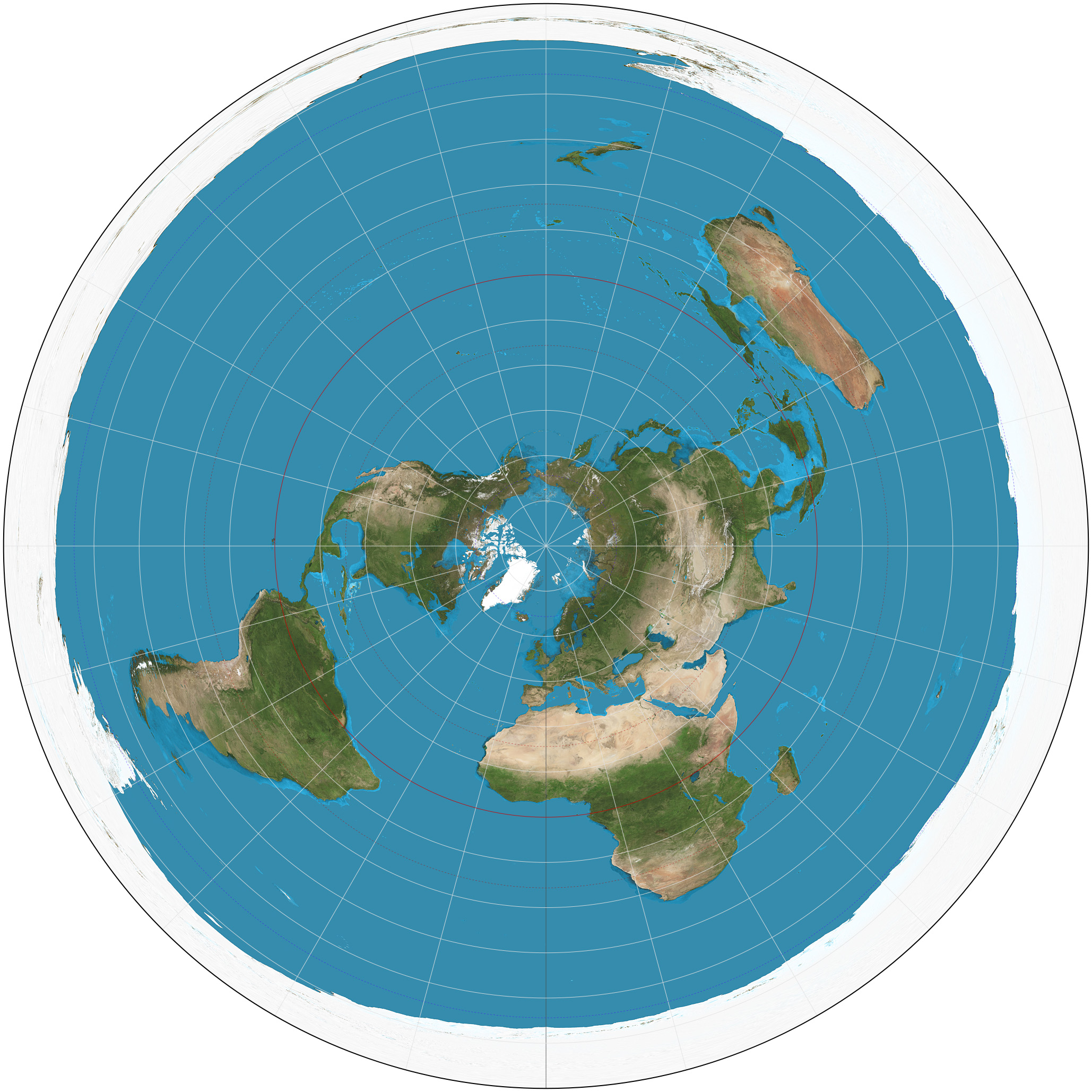
azimuthal projection interrupting the south pole

But most famous map projections interrupt the whole antimeridian in the Pacific ocean, including the poles.

I took a familiar but subtly different approach: I interrupt at the antimeridian, but excluding the poles. Therefore each non-pole point on the antimeridian has 2 copies: one for the western hemisphere, and one for the eastern. The extra copy isn't visible in my lattice diagrams, but it's there. Crossing the 180th line of longitude will therefore instantly transport you from the left side of the projection to the right. Many map projections interrupt the poles by converting them into lines, but I think that's a poor way to communicate shape. Points are points in my projections. Some other projections that do this are Mollweide and Hammer.

Transductive model

Most machine learning models you hear about are inductive. Using specific examples, they learn a general rule that converts from inputs to outputs. For instance, a cat vs. dog model may learn from 100,000 images and then be capable of classifying the practically infinite set of possible images.

But instead of an inductive model, I chose a transductive one, directly learning the output (projected xy coordinate) for each of my inputs (point on the sphere). Generalization just wasn't necessary for this application. The sphere is the only domain I care about. Plus, I didn't want to constrain myself to a parametrized model. By making every coordinate a parameter, I can learn any possible projection.

So technically, my "nonparametric" model has $2 * 3044 = 6088$ parameters; x and y coordinates for each point.

Loss function

This is an interesting part!

I'm measuring a local distortion at a point $p$ as the Jacobian $J_p$ of the projection from the sphere to the plane. To be clear: the Jacobian is computed using a local coordinate system with orthonormal basis vectors around $p$ , not from spherical coordinates.

This matrix $J_p$ has extremely useful singular values $\sigma_0$ and $\sigma_1$ . (The unofficial part 0 to this series, 6 Matrix Decompositions Everyone* Should Know, explains the singular value decomposition.)

The SVD converting a circle with axes v_0 and v_1 into an ellipse with axes
sigma_0 w_0 and sigma_1 w_1

The product $\sigma_0\sigma_1$ of $J_p$ 's singular values is the ratio by which the projection enlarges or shrinks areas, and the ratio $\sigma_0/\sigma_1$ of its singular values is related to the angular distortion. An angle on the sphere can differ from its projected counterpart by no more than $\left|\tan^{-1}\sqrt{\sigma_1/\sigma_0} - \tan^{-1}\sqrt{\sigma_0/\sigma_1}\right|$ radians. Each of these measures ( $\sigma_0\sigma_1$ and $\sigma_0/\sigma_1$ ) should ideally be 1.

By my reckoning, making something $r$ times too big is just as bad as making it $r$ times too small. Therefore, I applied the convex loss function $r + 1/r$ to each of these measures. I weighted them with some hyperparameter $\alpha$ and added them, giving

$\ell = \alpha\left(\sigma_0\sigma_1 + \frac1{\sigma_0\sigma_1}\right) + (1 - \alpha)\left(\frac{\sigma_0}{\sigma_1} + \frac{\sigma_1}{\sigma_0}\right)$

I summed this over each angle of triangle on the lattice, weighting by the product of the triangle's area and the angle. In this way, all lattice points get 360 degrees of angular weight, and all triangles get weight (almost exactly) in proportion to their area.

Optimization method

Grossly simplifying, there are 3 categories of optimization methods:

those where there's a simple mathematical structure to work with, such as a linear least squares problem,
those without a simple structure but where you can take gradients of the loss with respect to the model parameters, and
those where you can't even take gradients.

This problem falls into category 2. The loss function is complicated but differentiable, so gradient descent was a natural choice.

In particular, I used full-batch gradient descent with the Adam optimizer. Adam is an adaptive optimizer that adjusts per-parameter learning rate based on how noisy the recent gradients have been. I'm normally wary of adaptive optimizers, since they have peculiar dynamics which might not converge to a local minimum, no matter how small you set your learning rate. But in this case, Adam was overwhelmingly better than a plain gradient descent optimizer, since the loss was so much more sensitive to some coordinates than others.

See the difference over 600 iterations of training with tuned (non-exploding) learning rate:

Animation of
SGD optimized map projection learning (SGD)

Animation of
Adam optimized map projection learning (Adam)

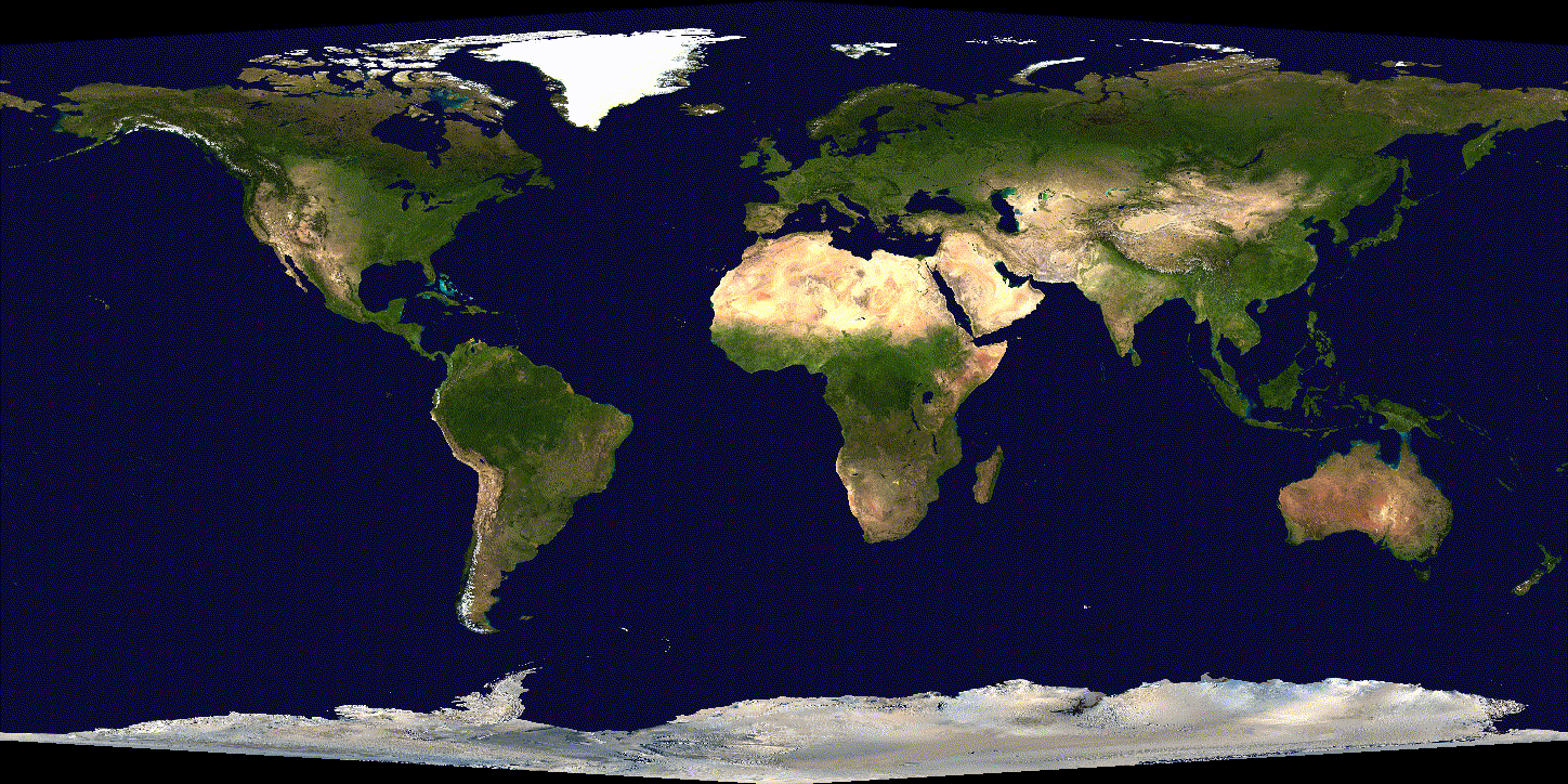
By the way, I'm using NASA's high resolution, true-color image of the Earth (confusingly named Blue Marble).

Software and Hardware

I implemented this in JAX and ran it on my Macbook Pro's M3 ~~GPU~~ (edit 2024-02-22: I realized there's something horribly wrong with jax-metal, the closed source library for using Apple silicon GPUs. Removing it and using the CPU improved my performance a whopping 300x.). The code is a mess right now, so I'll be making it available... later. Along with the learned projections.

Related Work

At first I searched for similar approaches to optimize non-parametric map projections, but couldn't find any. It was only by chance that I saw a Reddit post leading me to Justin Kunimune's Danseiji and Elastic projections. As far as I know, this is the only similar approach to mine. He has his own software project and paper, with some similar and some different decisions made. I only discovered it at the tail end of my research when I had already decided on most of my own approach.

It's a very cool piece of work, and he has quite a broad range of maps. His choice of L-BFGS is probably more efficient than gradient descent with Adam. If I have one criticism, though, it's that the Neo-hookean energy function doesn't seem to have physical meaning here. But I understand why he didn't choose the the Airy-Kavrayskiy criterion, which is similar to my loss function. Instead of the convex loss $r + 1/r$ , they use $\ln(r)^2$ , royally screwing up any hopes of a balanced loss distribution over the globe.

It's clear that Kunimune has some wisdom on this topic by now, saying

"With hindsight, I know that lenticular mesh-based projections (Danseiji N, I, and II) aren’t that good or interesting, and don’t gain you much you don’t already get from the Eckert or Györffy projections."

He's lost interest in the type of projection I'm making, but I am undeterred! In the next part, I'll start showing my results!

Map Projections 3: The Essential Results
Map Projections 4: Bullying the Oceans
Map Projections 5: More Interruptions

< previous next >