Graph all the things

analyzing all the things you forgot to wonder about

Map Projections 1: Not Solving Exactly

2023-09-28
interests: differential geometry, PDEs

I looked into whether it's mathematically possible to solve for an optimal map projection. That is - find a smooth bijective function from the sphere to a subset of the plane that minimizes the integral of a local loss function. The short answer: not for any interesting cases. I did solve one contrived example, though.

I'm saving the fun visualizations and flavor text for later posts. This one is just hard math.

Turning the optimization into a PDE

Every map projection can be thought of us a function $\mathbf{y}$ from spherical coordinates $(x_1, x_2)$ to euclidean coordinates $(y_1, y_2)$ (I'm using $x_1$ and $x_2$ instead of $\theta$ and $\phi$ to avoid some confusion later). Unfortunately, there's no perfect map projection that preserves both angles and area. All you can do is preserve one of these and keep the other one under control. Or you can forsake both and strike a compromise.

I thought about choosing a map projection as minimizing a local loss function integrated over the globe:

$\mathbf{y}_\text{opt} = \text{argmin}_{\mathbf{y}}\int_{\mathbf{x}\in X} w(\mathbf{x})\ell(D\mathbf{y}(x))$

where

$\mathbf{x} \in X$ are spherical coordinates,
$\mathbf{y}: X \to \mathbb{R}^2$ is a differentiable function from $X$ to the plane,
$D\mathbf{y}$ is the Jacobian of $\mathbf{y}(\mathbf{x})$ ,
$\ell: (\mathbb{R}^2 \times \mathbb{R}^2) \to \mathbb{R}$ is a smooth function for local loss given a Jacobian $J$ , and
$w(\mathbf{x}) = \sin x_2$ is a weight function to account for the local surface area of the sphere.

From here on, I'll be dropping arguments and letting $J$ be the Jacobian $D\mathbf{y}$ .

Optimizing a single parameter in $\mathbb{R}$ is intuitive.
Optimizing a function from $\mathbb{R}\to\mathbb{R}$ gets more interesting.
Optimizing a function from $\mathbb{R}^2\to\mathbb{R}^2$ is utterly confusing in my opinion. I worked out the following derivation.

A necessary condition for an optimal map projection is that applying a perturbation to it will not decrease the loss. If $\mathbf{\delta}$ is a smooth perturbation to $y$ ,

$\frac{d}{ds}\Bigg|_{s=0}\int_X w\ell(J + sD\mathbf{\delta}) = 0$

So, for each index $i$ ,

$\int_X w\left(\nabla_{J_i}\ell(J) \cdot \nabla_\mathbf{x}\delta_i\right) = 0$

where by $\nabla_{J_i}\ell$ , I mean "the gradient of $\ell$ with respect to the $i$ th column vector of its Jacobian argument. Using generalized integration by parts with $w\nabla_{J_i}\ell(J)$ and $\nabla_\mathbf{x}\delta_i$ as the parts, this turns into

$\int_{\partial X} \delta w \nabla_{J_i}\ell(J) \cdot \mathbf{n} - \int_{X} \delta \nabla_\mathbf{x} \cdot \left(w\nabla_{J_i}\ell(J)\right) = 0$

And now for the really powerful part! Since $\delta_i$ can be absolutely anything, the only way to satisfy this equation for all choices of $\delta_i$ is to make the rest of the integrands 0 everywhere:

$\forall i, x\in X, \qquad \nabla_\mathbf{x} \cdot \left(w\nabla_{J_i}\ell(J)\right) = 0 \qquad (1)$

$\forall i, x\in \partial X, \qquad w \nabla_{J_i}\ell(J) \cdot \mathbf{n} = 0 \qquad (2)$

Equation (1)'s simplest interpretation is something like, "there are no sinks or sources in the vector field of the weighted local loss gradient". This is a bit confusing because the loss gradient is with respect to changes in $y$ 's Jacobian, not to changes in $x$ , but the message is clear: if there were a sink, we could "move" some of $y$ into the sink (i.e. reduce $y$ in some places and increase it in others) to reduce loss.

Equation (2) specifies what the boundary of the projection should look like. Its interpretation is something like "when weight is nonzero, the gradient of loss with respect to the Jacobian must be perpendicular to the boundary". We must not be able to decrease loss by stretching the edges of the map projection in any direction.

This derivation reminds me a lot of Lagrangian mechanics. And there is certainly a differential geometry interpretation here, but I can't be bothered to sort it out.

But (1), the PDE, is quite troublesome. Choose pretty much any loss function, and it becomes utterly intractible. I will argue in a future blog post that the loss should be based on the singular values of $J$ , and simply expressing the demonic PDE arising from that is not worth anyone's time.

Instead, I'll solve a contrived example.

The contrived example

Finding a nontrivial solution to even (1) alone is hard, so instead I'll find a solution to (1) with a suboptimal boundary, not solving (2), using a simple loss function with a no-so-simple boundary condition.

Suppose we have this dumb $L^2$ loss:

$\ell(J) = ||J - I||^2$

This tries to make the map projection look as boring as possible: latitudes should look like horizontal lines, and longitudes should look like vertical ones. In fact, one can get the optimal loss of 0 via $\mathbf{y} = \mathbf{x}$ , the equirectangular projection. This projection's only merit is its mathematical simplicity.

But with the newfound derivation above, we can hunt for an optimal projection under this loss with a non-rectangular shape. Starting from (1), plugging everything in, and skipping the intermediate work, we get a PDE for each of $y_1$ and $y_2$ :

$\sin x_2 \left(\frac{\partial^2 y_1}{\partial x_1^2} + \frac{\partial^2 y_1}{\partial x_2^2}\right) + \cos x_2 \frac{\partial y_1}{\partial x_2} = 0$

$\sin x_2 \left(\frac{\partial^2 y_2}{\partial x_1^2} + \frac{\partial^2 y_2}{\partial x_2^2}\right) + \cos x_2 \left(\frac{\partial y_2}{\partial x_2} - 1\right) = 0$

There are a lot of solutions to these - one for every boundary condition. Most of them are utterly incomprehensible, but here's a clean one (for some constants $a$ , $b$ , $c$ ):

$y_1 = a(x_1 + b)\left(1 + c\left|\ln\tan\left(\frac{x_2}{2}\right)\right|\right)$

$y_2 = x_2$

Choosing $a=0.4$ , $b=-\pi$ , $c=1$ and plotting between $\pm85^\circ$ latitude gives this:

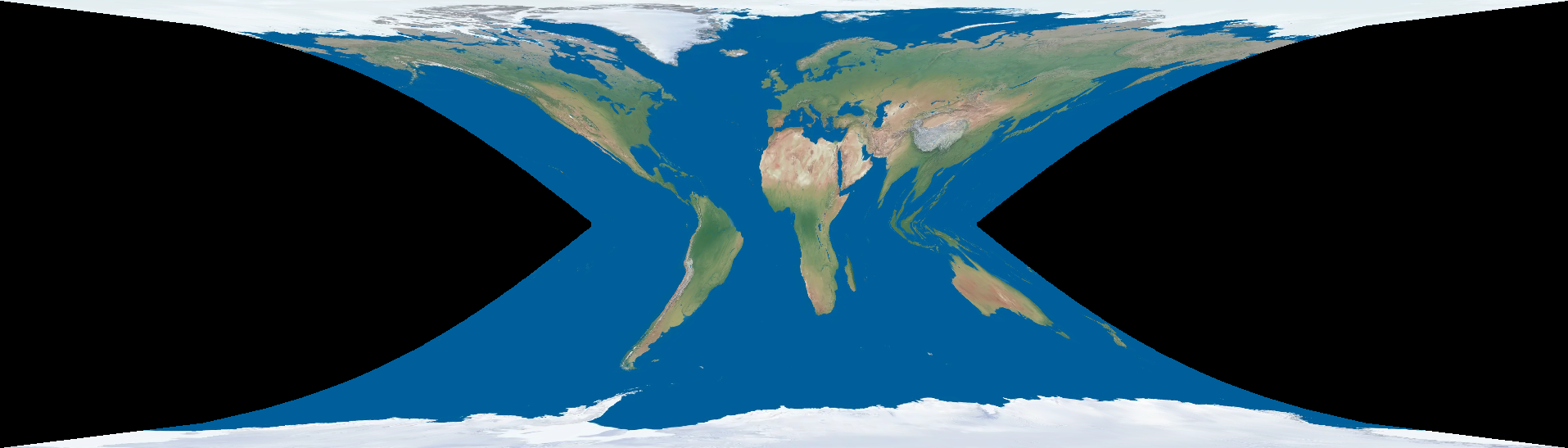
first inscrutable diagram from original paper

So... yeah, we have a map projection that's optimal (by a silly definition) everywhere (except the ridiculous boundary). In that very lame sense, we can exactly solve some optimal map projections.

In future parts, I'll look at the more interesting technique of solving optimal map projections numerically.

Map Projections 2: Solving Numerically
Map Projections 3: The Essential Results
Map Projections 4: Bullying the Oceans
Map Projections 5: More Interruptions

< previous next >